经典白忙活
线性回归模型的假设空间相当有限,为了让我们的模型更加适应普遍的情况,我们可以引入更加丰富多变的假设,即高斯过程。
Kernel Regression
In order to work with a GP it makes sense to write a bit more sensible structured code and break up a few things into functions. The first thing we want to implement is a function that allows us to compute the covariance matrix. It could be nice to try and modularise this so that you can easily use your code with several different covariance functions.
为了实现GP功能,我们首先要做的事情是计算出样本的协方差矩阵,而获得这个矩阵的最佳方法,便是利用Kernel Regression,下方就是基于Kernel Regression编写的求协方差的函数,varSigma控制函数垂直方向的波动性,lengthscale控制函数的平滑度,这个函数可以求得点集x1和x2的协方差:
def rbf_kernel(x1, x2, varSigma, lengthscale):
    if x2 is None:
        d = cdist(x1, x1)
    else:
        d = cdist(x1, x2)
    K = varSigma*np.exp(-np.power(d, 2)/lengthscale)
    return K

#    Args:
#        X1: ndArray, m个点 (m x d).
#        X2: ndArray, n个点 (n x d).
#    返回:
#        协方差矩阵 (m x n).
我们也可以针对这个函数,赋一些比较简单的值,进行一些test:
x = np.linspace(-5, 5, 200).reshape(-1, 1)
c=x.shape
# compute covariance matrix
K = rbf_kernel(x, None, 1.0, 2.0)
# create mean vector
mu = np.zeros(c[0])
# draw samples 20 from Gaussian distribution
f = np.random.multivariate_normal(mu, K, 20)
fig = plt.figure()
ax = fig.add_subplot(111)
ax.plot(x, f.T)
plt.show()
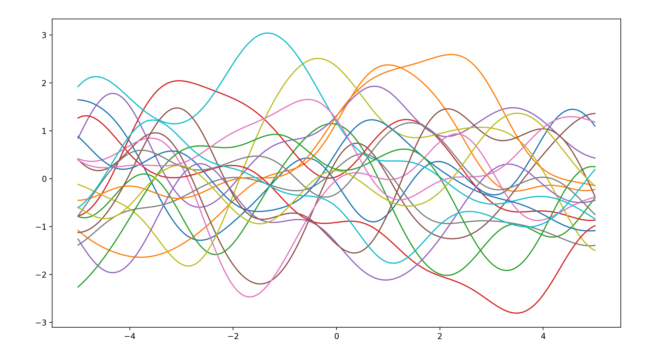
当varSigma=1.0,lengthscale=2.0时:
得出如下的函数曲线,接下来我们将使用这个曲线作为基准值进行对比:
当varSigma=1.0,lengthscale=50.0时:
得出如下的函数曲线:
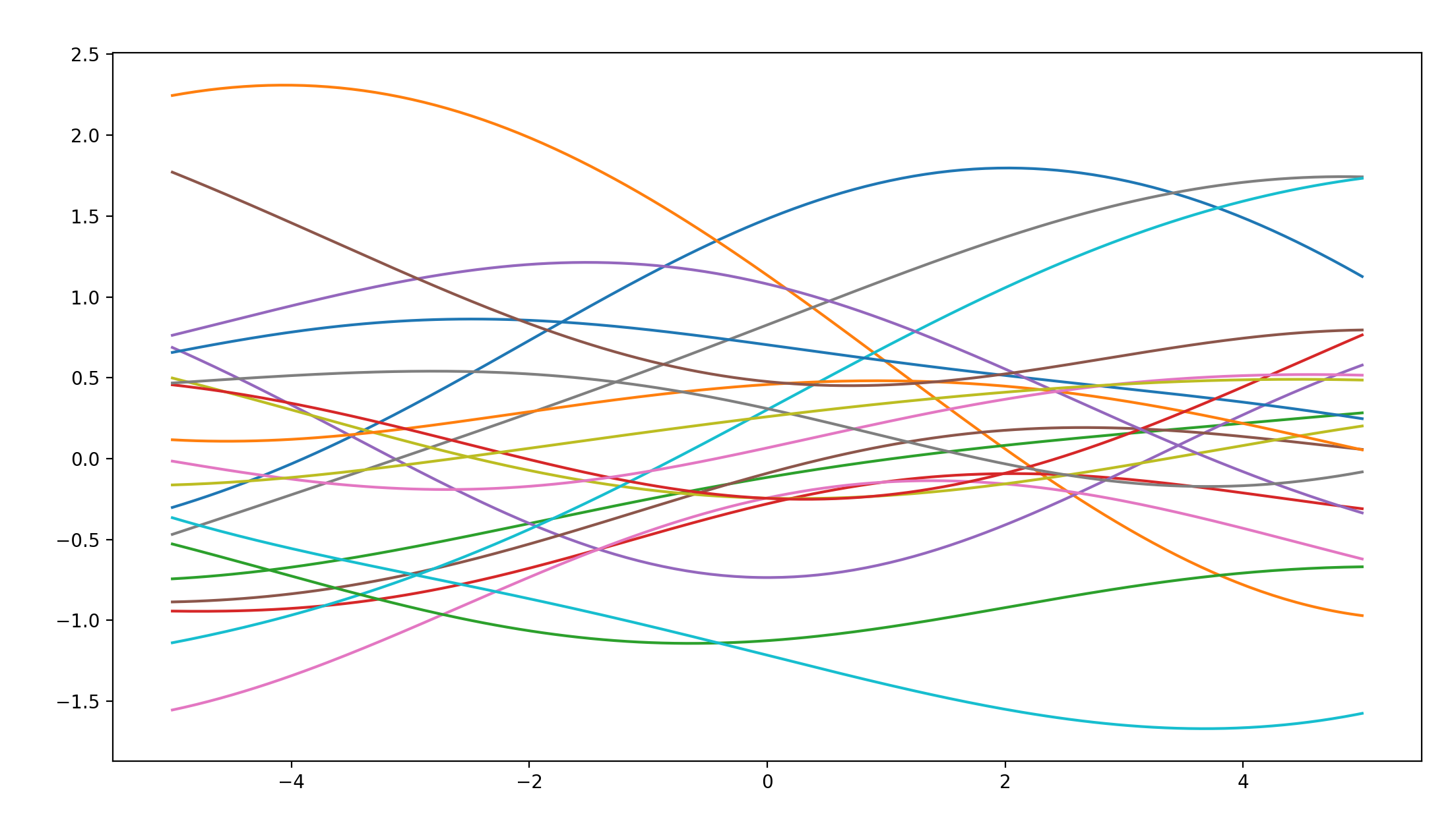
不难看出,在lengthscale参数较大时,函数的平滑度相较于第一幅函数图像有了很大的提升。
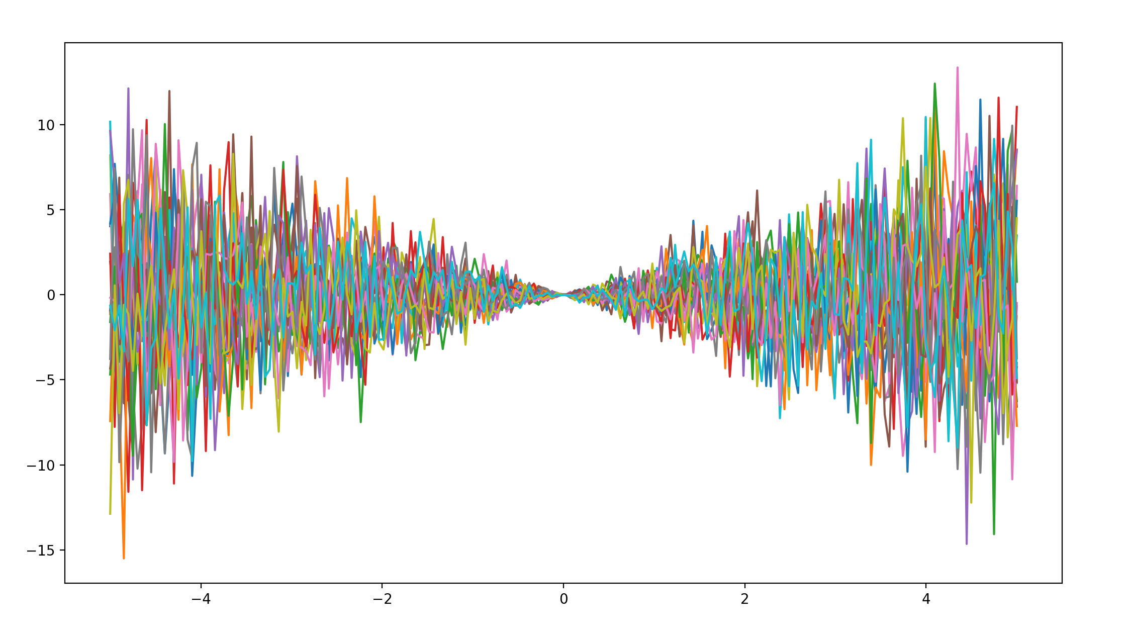
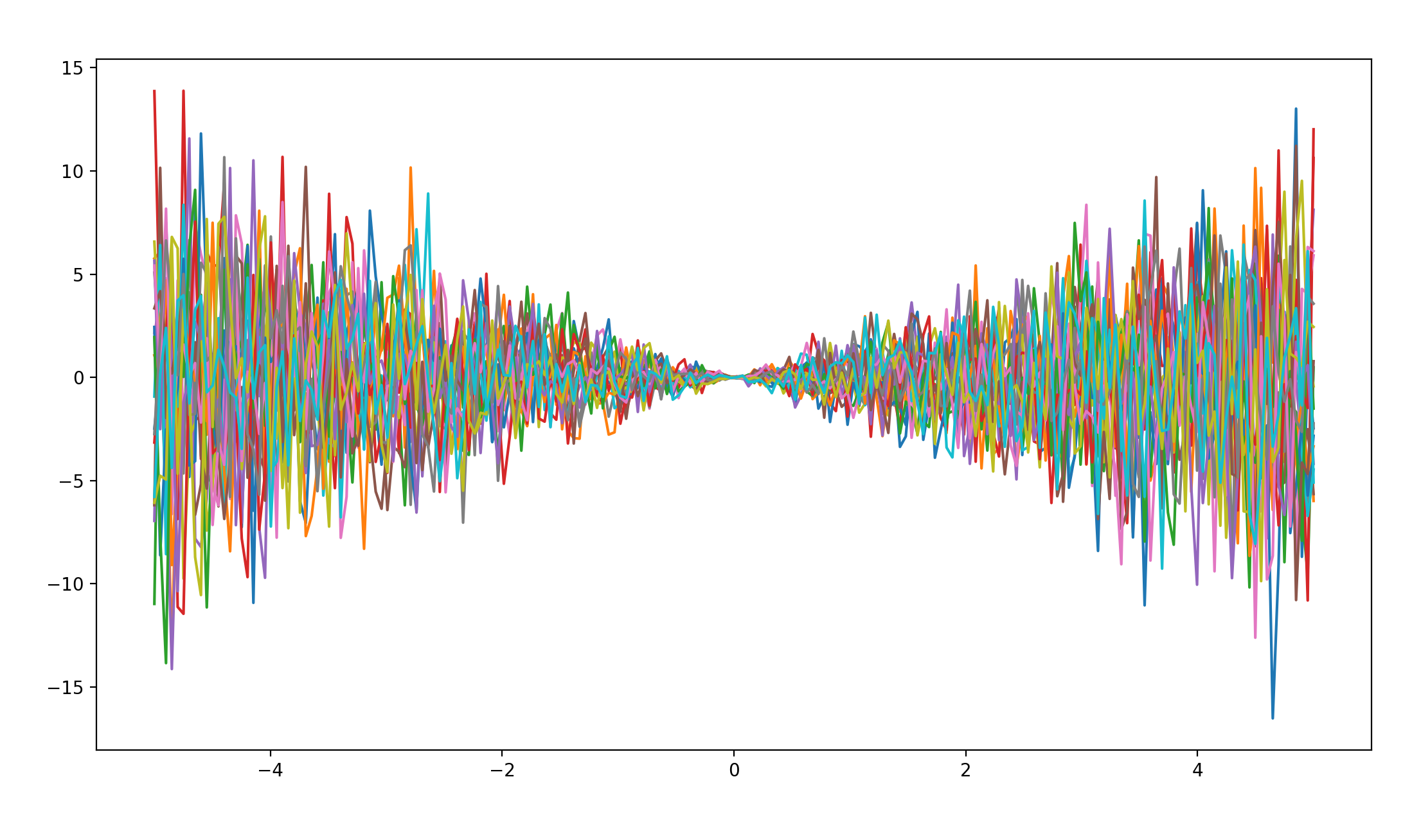
当varSigma=10.0,lengthscale=2.0时:
得出如下函数曲线:
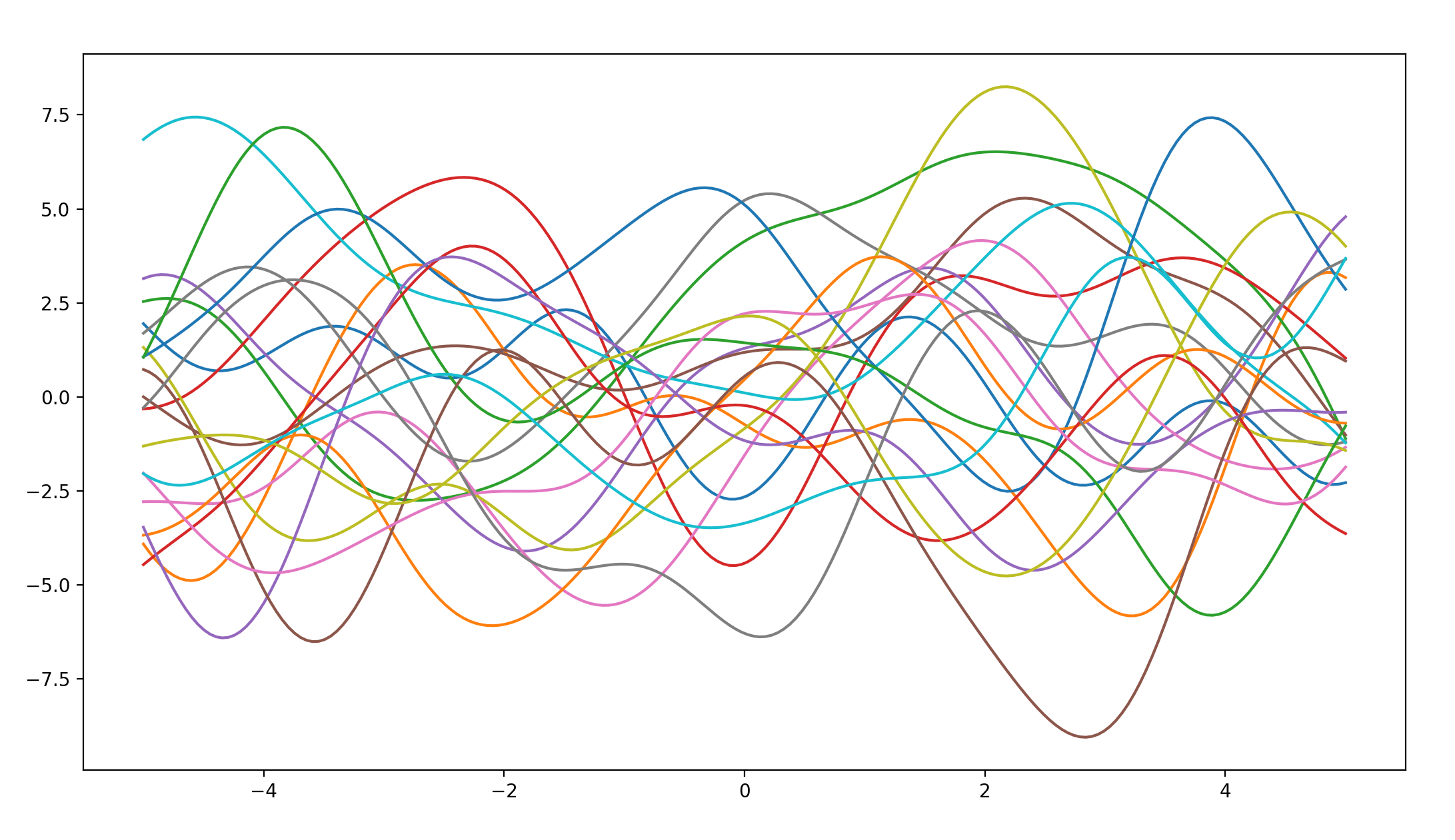
不难看出,在varSigma参数较大时,函数的纵坐标总体都有了一定程度的增大,说明函数在垂直方向的波动性提升了。
先验分布
The important thing to understand is that even if the process is infinite, as are the number of values the function can be evaluated across, due to the consistency of a GP we can decide to only look at a finite subset of the process. This is what we define using x. Test to increase and decrease the cardinality of the index set. Sampling from the prior is very important as it allows us to see what assumptions we can encode with the parameters. Importantly, the GP places non-zero probability on every function so if you sample for long enough everything will appear, with a few samples you are only seeing the most likely things.
由于GP在每个函数上都放置了一个非零的概率,所以,在时间允许的情况下,任何形状的函数都可以被采样到,所以,提供一个合适的先验分布来缩小置信空间就显得十分必要了。
Now lets try to change the covariance function and see how the samples change, lets implement three more covariance functions, a white-noise, a linear and a periodic covariance.
接下来还有三个另外的协方差函数,我们一次对他们进行测试:
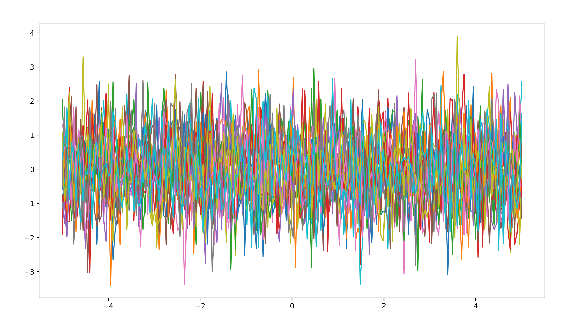
测试参数:varSigma=1.0,lengthscale=2.0,period=2
white-noise covariance
def white_kernel(x1, x2, varSigma):
    if x2 is None:
        return varSigma*np.eye(x1.shape[0])
    else:
        return np.zeros(x1.shape[0], x2.shape[0])
函数图像如下:
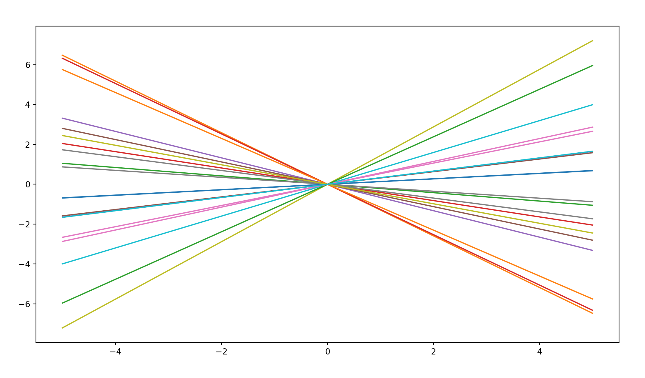
linear covariance
def lin_kernel(x1, x2, varSigma):
    if x2 is None:
        return varSigma*x1.dot(x1.T)
    else:
        return varSigma*x1.dot(x2.T)
函数图像如下:
periodic covariance
def periodic_kernel(x1, x2, varSigma, period, lenthscale):
    if x2 is None:
        d = cdist(x1, x1)
    else:
        d = cdist(x1, x2)
    return varSigma*np.exp(-(2*np.sin((np.pi/period)*d)**2)/lenthscale**2)
函数图像如下:
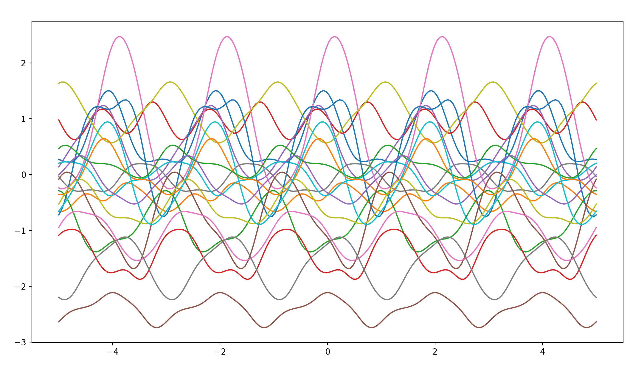
通过对这些图像的观察,我们可以发现不同的协方差函数生成的对应函数图像的特点。
不仅如此,我们除了可以观察不同函数图像的特点外,还可以将不同的协方差结果相乘,观察函数图形的特点:
periodic covariance * linear covariance
函数图像如下:
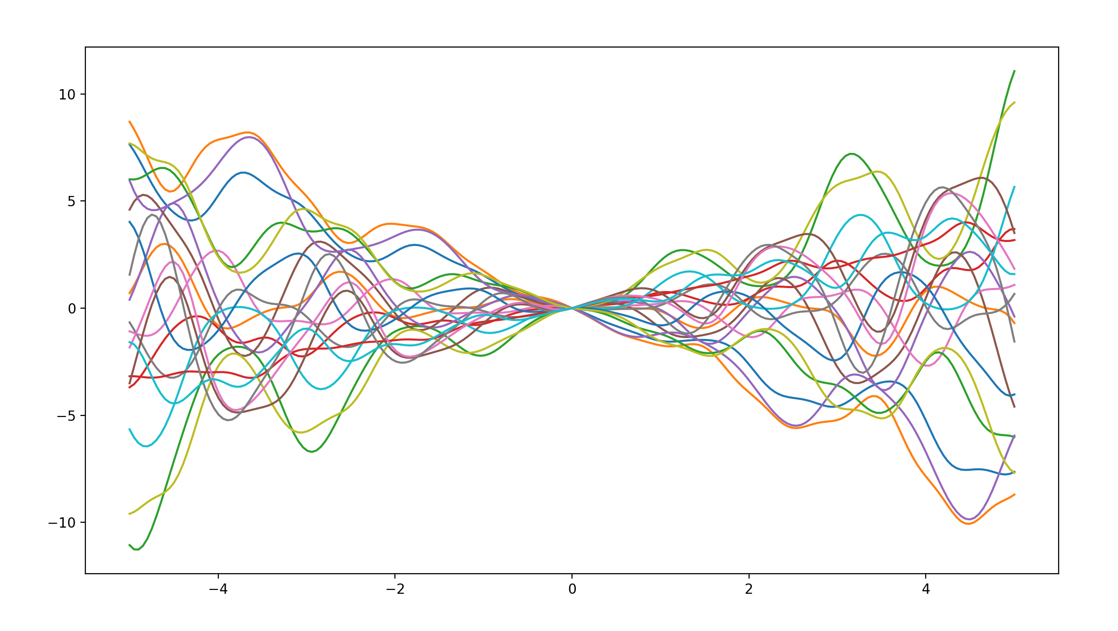
通过观察我们不难发现,这个图像综合了两个协方差图像的特点,既具有线性,在某方向也具有一些周期性,so funny。
periodic covariance * white-noise covariance
函数图像如下:
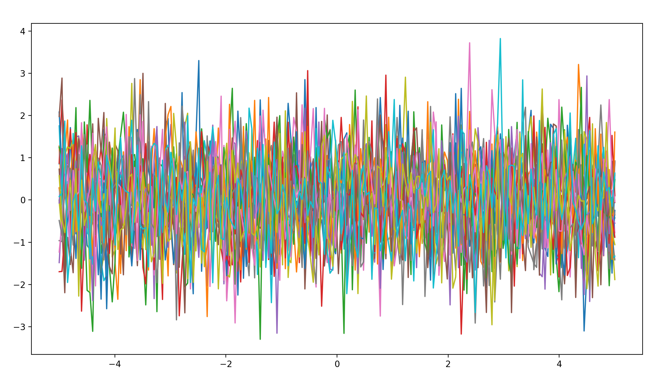
哈哈哈哈哈,由于白噪音本身就是杂乱无章的,这幅图像似乎与white-noise covariance单独作用的区别并不大,既然white-noise covariance的影响如此之大,不让让它和linear covariance组合一下,看看会产生什么结果,是否还会像这次一样直接被white-noise covariance同化。
linear covariance * white-noise covariance
函数图像如下:
哈哈,猜中了,但没完全猜中,这幅图像既继承了white-noise covariance的杂乱性,也保留了linear covariance的线性,由于linear covariance的线性,整幅图像才展现出了这样的杂乱这向两侧发散的图形。
做一个小小的预测,如果我将这三个结果乘在一起,图像形状应该与这幅图类似,纵坐标绝对值稍大,因为periodic covariance的周期性完全被white-noise covariance抵消了。
linear covariance * white-noise covariance * periodic covariance
函数图像如下:
嘿嘿,对喽。
后验分布
In specific a GP is definedas a infinite collection of random variables which are all jointly Gaussian distributed. So lets make use of this. Lets assume that we have observed data D and now we want to predict what the output of the function is at locations x∗
假设我们已经获得了数据集D,我们要通过这个数据预测出函数的位置,这时可以将联合分布写为:
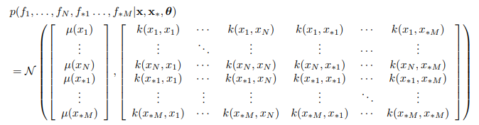
其中 µ(·) 和 k(·,·) 是均值和协方差函数,θ 是后者的参数,我们可以利用乘积规则来处理我们的联合分布。
我们不妨先利用下方代码随机生成一些点,并计算一下后验分布,观察这些已知的点会对我们的后验分布函数图形造成什么烟的影响。
N为随机生成点的个数
N = 5
x = np.linspace(-3.1,3,N)
y = np.sin(2*np.pi/x) + x*0.1 + 0.3*np.random.randn(x.shape[0])
x = np.reshape(x,(-1,1))
y = np.reshape(y,(-1,1))
x_star = np.linspace(-6, 6, 500).reshape(-1,1)
我们不妨先忽略高斯噪声影响,编写基于Gausasian Regression的后验分布计算函数:
def gp_prediction(x1, y1, xstar, lengthScale, varSigma):
    k_starX = rbf_kernel(xstar,x1,lengthScale,varSigma)
    k_xx = rbf_kernel(x1, None, lengthScale, varSigma)
    k_starstar = rbf_kernel(xstar,None,lengthScale,varSigma)
    mu = k_starX.dot(np.linalg.inv(k_xx)).dot(y1)
    var = k_starstar - k_starX.dot(np.linalg.inv(k_xx)).dot(k_starX.T)
    return mu, var, xstar
生成五十个后验分布函数,绘出可视化图形:
Nsamp = 50
mu_star, var_star, x_star = gp_prediction(x, y, x_star, lengthScale, varSigma)
# print (mu_star)
# print("separate")
# print(var_star)
# print("separate")
# print(x_star)
mu_star=np.squeeze(mu_star)
f_star = np.random.multivariate_normal(mu_star, var_star, Nsamp)
fig = plt.figure()
ax = fig.add_subplot(111)
ax.plot(x_star, f_star.T)
ax.scatter(x, y, 200, 'k', '*', zorder=2)
plt.show()
当无已知点时
函数图形如下所示:
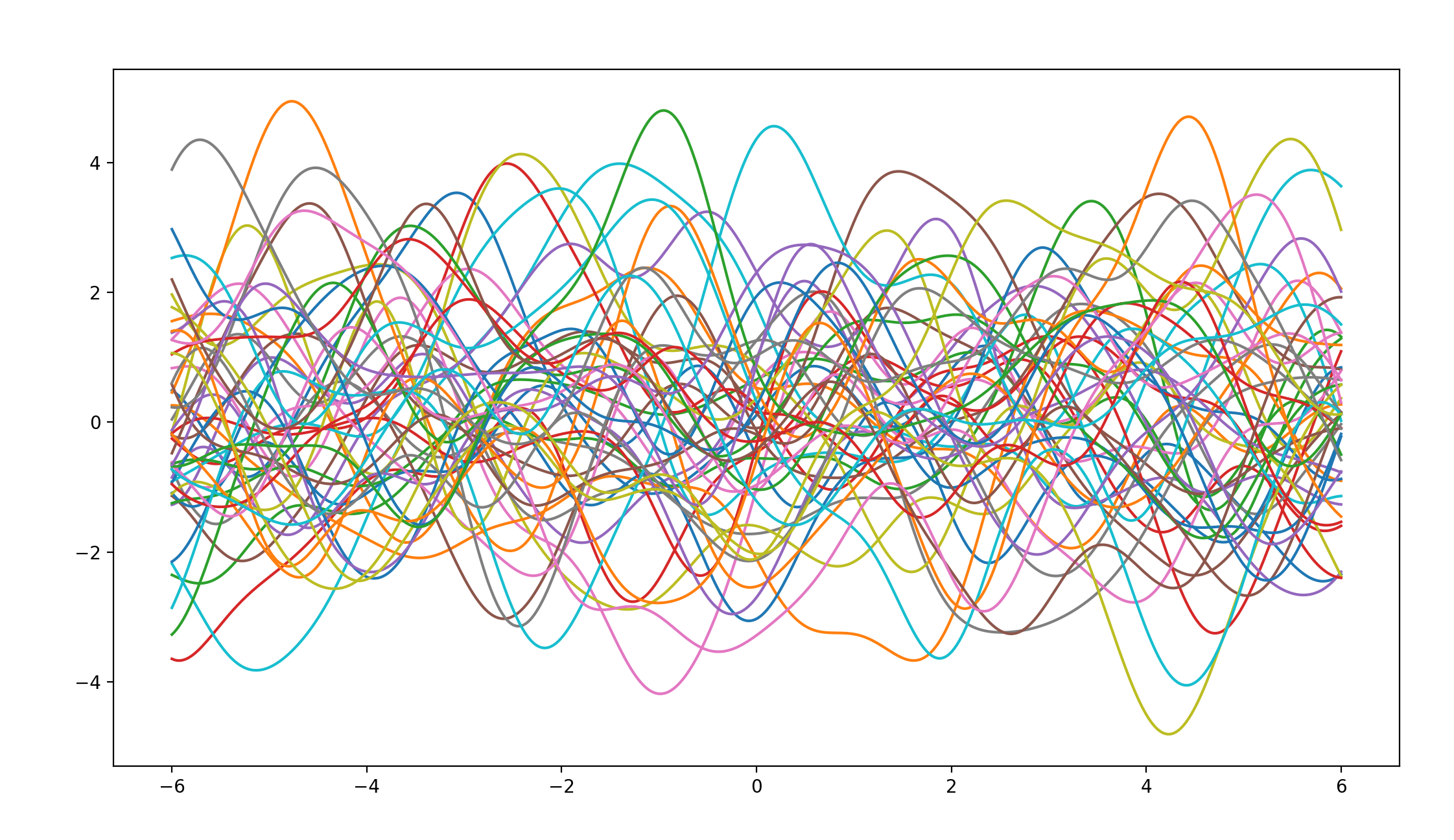
不难看出,在无已知点时,各个后验分布函数图像是杂乱无章毫无规律可言的。
当有五个已知点时
函数图像如下所示:
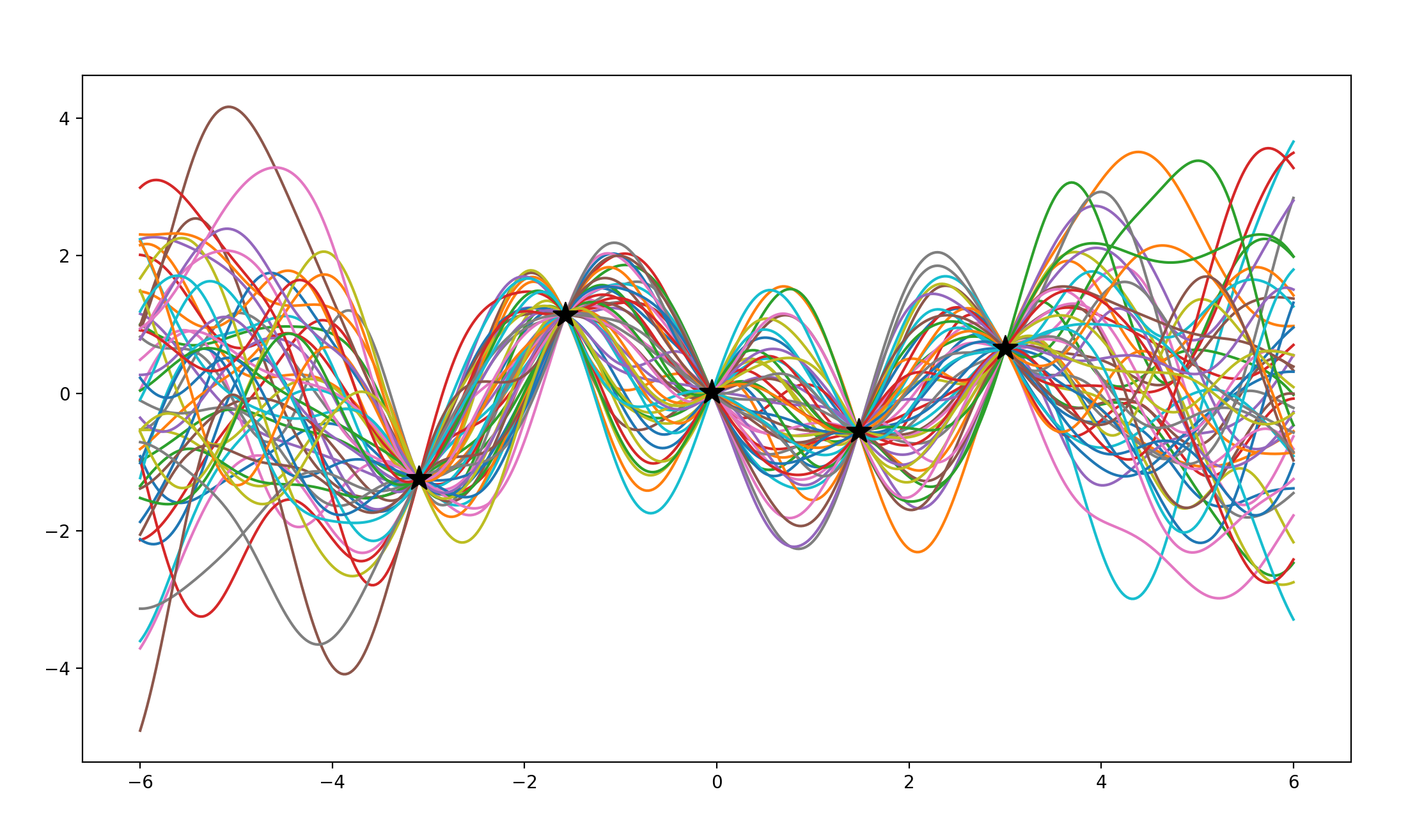
虽然整体还是偏于无序,但在已知的五点处以及点与点之间呈现了收敛的趋势,不难总结出,已知点让后验分布趋向归一。
当有十个已知点时
函数图像如下所示:
不难看出,所给的已知点越多,函数图像越趋向于归一,在长度为12的定义域内给定十个已知点,已经可以让后验分布函数图像有一个很不错的收敛。
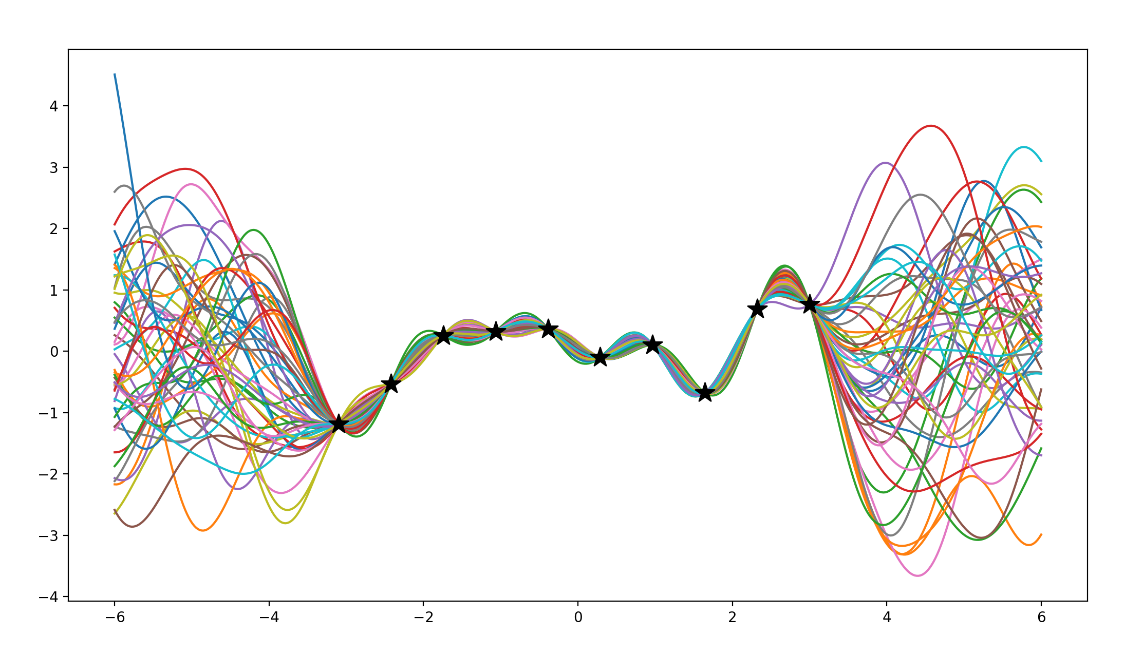
当有十个以上已知点时
部分函数图像如下所示:
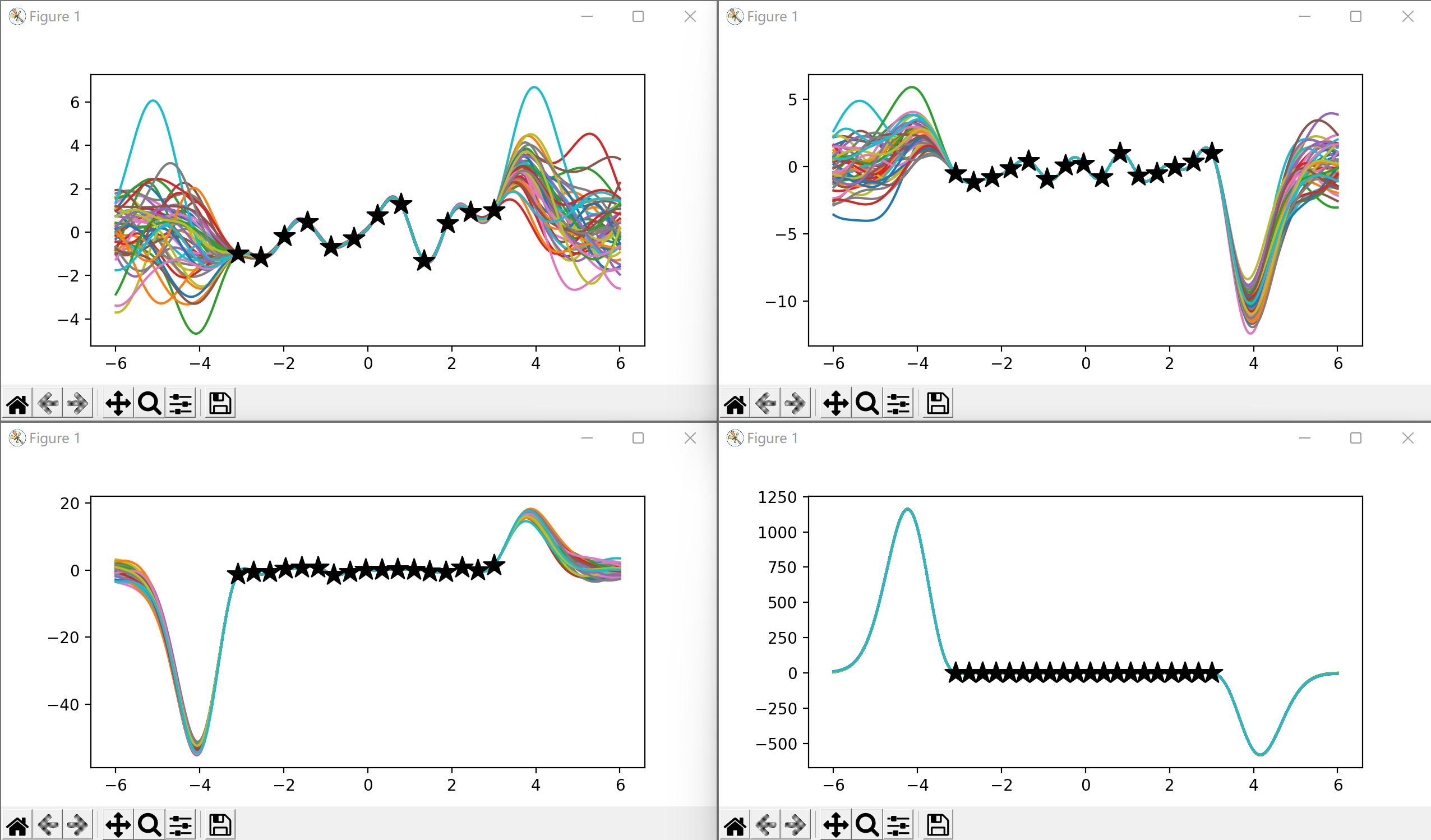
随着已知点的增加,函数图像的收敛性不断增强,后验分布函数图像不断收敛,最后几乎收敛成一条线。不仅在比较大的纵坐标分度值下如此,在我对图像进行缩放使分度值统一时结果依然如此,五十条曲线几乎拟合成为同一条。 当然,在如此小的定义域内有如此多的数据在现实中是很难实现的。
点集的均值和方差
©著作权归作者所有